利用深度学习技术可以实现对特定动物的识别，具有重大意义

本文方法

NMYOLO官方对于yolov8进行了详细的图解，如果你感兴趣的话，可以进入下面的链接查看

mmyolo/configs/yolov8/README.md at dev · open-mmlab/mmyolo · GitHub

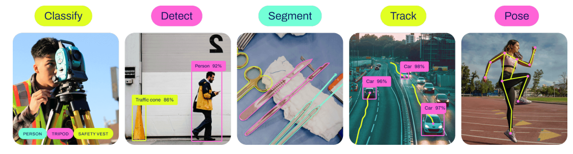
Ultralytics开发的YOLOv8是一款尖端、最先进（SOTA）的模型，它借鉴了之前YOLO版本的成功经验，并引入了新的特性和改进，以进一步提高性能和灵活性。YOLOv8旨在实现快速、准确和易于使用，因此是各种目标检测、图像分割和图像分类任务的绝佳选择。除了支持最经典的目标检测任务之外，还添加了对语义分割、分类和追踪等任务的支持。

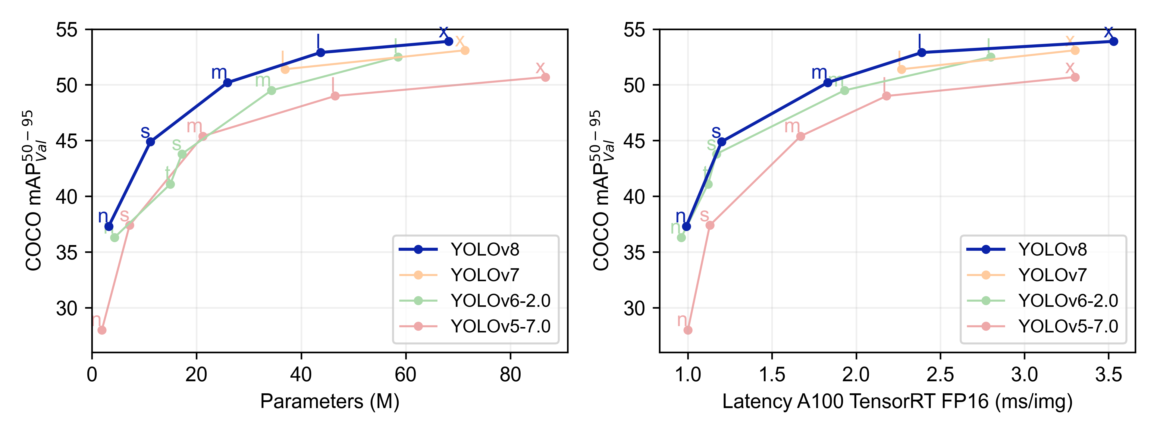
首先来看一下YOLOv8算法的性能.根据官方提供的性能图，其中左图的横坐标表示的是网络的参数量，右图的横坐标表示的网络在A100显卡上的推理速度，纵坐标方面表示表示的都是模型的精度。可以看到，YOLOv8模型的在同样的参数量下，比其他系列的YOLO模型有明显的精度提升，在右图展示的同样的map精度下，YOLOv8的模型也同样有更快的速度，还就那个更高、更快、更强

总的来说，yolov8算法的核心点在于

1. 给出了一个全新的视觉模型，保持精度的同时，实现了较高的检测速度，并且同时支持支持图像分类、物体检测和实例分割等多种视觉任务。并且根据卷积层提供了多个规模的模型（nano、small、medium、large和x-large），满足用户不同场景的需要。

2. 新的骨干网络：YOLOv8引入了一个新的骨干网络，可能参考了YOLOv7 ELAN设计思想，将YOLOv5中的C3结构换成了梯度流更丰富的C2f结构，并对不同尺度模型调整了不同的通道数，大幅提升了模型性能。

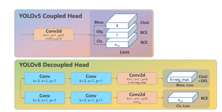
3. 解耦头的设计：YOLOv8的Head部分从原先的耦合头变成了解耦头结构，将分类和检测头分离，并且从Anchor-Based转变为Anchor-Free，简化了模型结构并提高了推理速度。

4. 新的损失函数：YOLOv8在Loss计算方面采用了TaskAlignedAssigner正样本分配策略，并引入了Distribution Focal Loss，确保了检测结果的准确性和鲁棒性。

结构说明

根据NMYOLO给出图可以知道

其中Backbone是骨干网络部分·，主要是做特征提取，从这个网络中可以提取出三个不同尺度的特征出来，然后送入Neck部分，Neck部分主要是做一些融合，融合之后的特征会送入Head部分做进一步的解码，解码的部分分为两个部分，一个是bonding box（边界框的解码）另一个是Class loss（分类的解码）

骨干网络部分

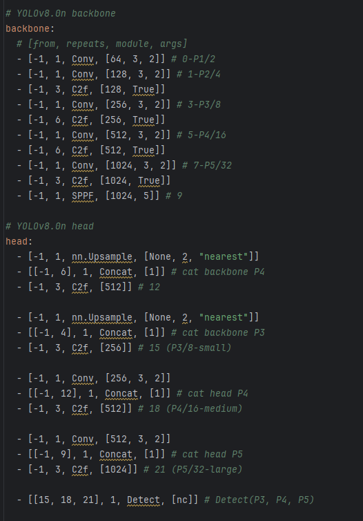
骨干网络的配置文件如下所示：

下面的图是YOLO模型原先使用的C3结构和新的C2f的结构。

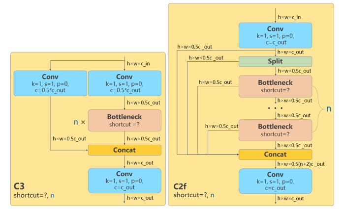
其中C3表示使用常规的三个卷积模块，c2f表示使用了2个卷积模块并且更快（fast），在不改变原始架构和梯度传输路径的前提下，使用分组卷积踢来以及使用洗牌和合并的操作组合不同组的特征，增强模型从不同特征图中的学习能力，达到改善参数的作用。和左图相比，增加了更多的跳层的连接和split操作。从源码中可以看出，对于原先的结构而言，只使用了一次cat操作，对于c2f结构而言，使用了多次的split操作和cat操作，按照原文的说法是增加了梯度流。

class C3(nn.Module):
"""
这里是使用了3个卷积层的csp结构
CSP Bottleneck with 3 convolutions.
"""
   def __init__(self, c1, c2, n=1, shortcut=True, g=1, e=0.5):
"""Initialize the CSP Bottleneck with given channels, number,
shortcut, groups, and expansion values."""
       super().__init__()
       c_ = int(c2 * e) # hidden channels
       self.cv1 = Conv(c1, c_, 1, 1)
       self.cv2 = Conv(c1, c_, 1, 1)
       self.cv3 = Conv(2 * c_, c2, 1) # optional act=FReLU(c2)
       self.m = nn.Sequential(*(Bottleneck(c_, c_, shortcut, g, k=((1, 1),(3, 3)), e=1.0) for _ in range(n)))
   def forward(self, x):
"""Forward pass through the CSP bottleneck with 2 convolutions."""
       return self.cv3(torch.cat((self.m(self.cv1(x)), self.cv2(x)), 1))

class C2f(nn.Module):
"""
这里使用了分支处理的操作，使用的是通过关闭残差链接的方式实现
先进行分支的操作然后再进行特征融合的操作
Faster Implementation of CSP Bottleneck with 2 convolutions.
"""
   def __init__(self, c1, c2, n=1, shortcut=False, g=1, e=0.5):
"""Initialize CSP bottleneck layer with two convolutions with
arguments ch_in, ch_out, number, shortcut, groups,
expansion.
"""
       super().__init__()
       self.c = int(c2 * e) # hidden channels
       self.cv1 = Conv(c1, 2 * self.c, 1, 1)
       self.cv2 = Conv((2 + n) * self.c, c2, 1) # optional act=FReLU(c2)
       self.m = nn.ModuleList(Bottleneck(self.c, self.c, shortcut, g, k=((3,3), (3, 3)), e=1.0) for _ in range(n))

   def forward(self, x):
"""Forward pass through C2f layer."""
       y = list(self.cv1(x).chunk(2, 1))
       y.extend(m(y[-1]) for m in self.m)
       return self.cv2(torch.cat(y, 1))

   def forward_split(self, x):
"""Forward pass using split() instead of chunk()."""
       y = list(self.cv1(x).split((self.c, self.c), 1))
       y.extend(m(y[-1]) for m in self.m)
       return self.cv2(torch.cat(y, 1))

解码头部分

解码头部分选择了使用分类的解码头，即边界框回归和分类分别作为两个分支处理。在原解码头部分，上图显示了经过主干网络提取特征后的特征图，直接进入解码模块，包含边界框回归的CIoU、置信度计算的obj和分类类别计算的CLS。改进后的解码头如下图所示，经过主干网络提取特征后，上方分支用于回归，下方分支用于分类，去除了之前的obj部分。在回归分支中，采用了Distribution Focal Loss。

DFL损失函数的定义如下：在训练过程中，目标的边界框被视为一个分布而非确定的数值。以浪花物体为例，其边界并非清晰可辨，而是模糊不定的。通过这样的损失函数设计，可以有效减少网络在训练过程中出现过拟合现象，提高模型的泛化能力。

实现的代码如下，这个函数实现了 Distribution Focal Loss (DFL)，用于学习密集目标检测中的合格和分布式边界框。通过计算目标距离标签的左右边界，并结合交叉熵损失，计算出最终的损失值。

def distribution_focal_loss(pred, label):
    r"""Distribution Focal Loss (DFL) is from `Generalized Focal Loss:
    Learning Qualified and Distributed Bounding Boxes for Dense Object Detection
    <https://arxiv.org/abs/2006.04388>`_.

    Args:
        pred (torch.Tensor): Predicted general distribution of bounding boxes
            (before softmax) with shape (N, n+1), n is the max value of the
            integral set `{0, ..., n}` in paper.
        label (torch.Tensor): Target distance label for bounding boxes with
            shape (N,).

    Returns:
        torch.Tensor: Loss tensor with shape (N,).
    """
    # label为y, pred为y^(y的估计值）
    # 因为y_i <= y <= y_i+1(paper)
    # 取dis_left = y_i, dis_right = y_i+1
    dis_left = label.long()
    dis_right = dis_left + 1

    weight_left = dis_right.float() - label  # y_i+1 - y
    weight_right = label - dis_left.float()  # y - y_i

    # paper中的log(S)这里用CE
    loss = (
        F.cross_entropy(pred, dis_left, reduction="none") * weight_left
        + F.cross_entropy(pred, dis_right, reduction="none") * weight_right
    )

    return loss

损失函数

YOLOv8的损失计算包括分类和回归两个部分，不再包含之前的目标置信度分支。分类分支采用二元交叉熵损失（BCE Loss），回归分支则采用了两个部分：Distribution Focal Loss和CIoU Loss。这三个损失函数按照设定的权重比例进行加权计算，为模型的训练提供了更精确和全面的指导。

在YOLOv8中采用了TOOD的TaskAlignedAssigner策略，该策略是一种动态分配对象的方法，根据分类和回归的分数加权来选择正样本。这种匹配策略的简单总结为：根据物体在分类和回归任务中的得分情况，来选取正样本，以提高模型在目标检测任务中的准确性和效率。

数据增强

数据增强在YOLOv8中得到了进一步的加强，继承了YOLOv5的颜色变换、马赛克数据增强和随机剪切等一系列传统方式，并引入了YOLOX的数据增强策略。与以往不同的是，在训练的前期阶段充分利用数据增强技术，而在接近尾声的最后10个epoch中则关闭数据增强，以达到更好的训练效果。

训练策略说明

YOLOv8在推理过程中与YOLOv5几乎一模一样，唯一的区别在于对Distribution Focal Loss中的积分表示bbox形式进行解码，转换成常规的4维bbox形式，接下来的计算过程与YOLOv5相似。以COCO的80类为例，假设输入图片尺寸为640x640，在MMYOLO实现中的推理过程如下所示：

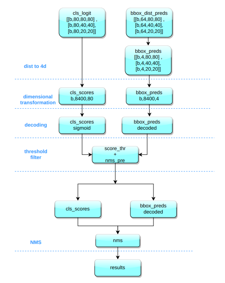
将bbox的积分形式通过Softmax和Conv转换为4维bbox格式，对Head输出的bbox分支进行处理。
YOLOv8输出的特征图包括尺度为80x80、40x40和20x20的三个特征图。Head部分输出分类和回归共6个尺度的特征图，将不同尺度的类别预测分支和bbox预测分支进行拼接，并进行维度变换。类别预测分支和bbox预测分支的形状分别为(b,8400,80)和(b,8400,4)，为了后续处理方便，将通道维度置换到最后。
对分类预测分支进行Sigmoid计算，对bbox预测分支进行解码，还原为真实的原图解码后的xyxy格式。
在遍历batch中的每张图时，使用score_thr进行阈值过滤，考虑multi_label和nms_pre，确保过滤后的检测框数量不会超过nms_pre。
将剩余的检测框还原到网络输出前的原图尺度，然后进行nms处理。最终输出的检测框数量不会超过max_per_img。

实操：实验配置

理论上如果要应用在V5、V7等其他版本，只需要稍微修改下配置文件即可。

注意，以下所有的配置基于我自己的代码文件，如果你需要可以联系我(*^_^*)

推荐该项目使用Anaconda+Pycharm组合使用，使用Anaconda创建虚拟环境（毕竟每一个项目所依赖的版本不同），并且在Pycharm中可以方便管理工程项目文件和使用conda虚拟环境

使用Anaconda创建一个虚拟环境之前，务必进行国内源切换，不然有些包的安装会很麻烦

conda config --remove-key channels
conda config --add channels
https://mirrors.tuna.tsinghua.edu.cn/anaconda/pkgs/free/
conda config --add channels
https://mirrors.tuna.tsinghua.edu.cn/anaconda/pkgs/main/
conda config --add channels
https://mirrors.tuna.tsinghua.edu.cn/anaconda/cloud/pytorch/
conda config --set show_channel_urls yes
pip config set global.index-url https://pypi.tuna.tsinghua.edu.cn/simple

创建虚拟环境(使用的Python版本是3.8.5)后，利用Pycharm打开工程文件，并将python解释器换成conda的虚拟环境，随后安装pytorch

conda install pytorch==1.8.0 torchvision torchaudio cudatoolkit=10.2 # 注意这条命令指定Pytorch的版本和cuda的版本，10系显卡
conda install pytorch==1.10.0 torchvision torchaudio cudatoolkit=11.3 # 30系列以上显卡gpu版本pytorch安装指令
conda install pytorch==1.8.0 torchvision==0.9.0 torchaudio==0.8.0 cpuonly #仅CPU的执行这条命令即可

cd进入到pyproject.toml文件所在的路径，安装其他依赖库

pip install -v -e .

训练自己的数据集

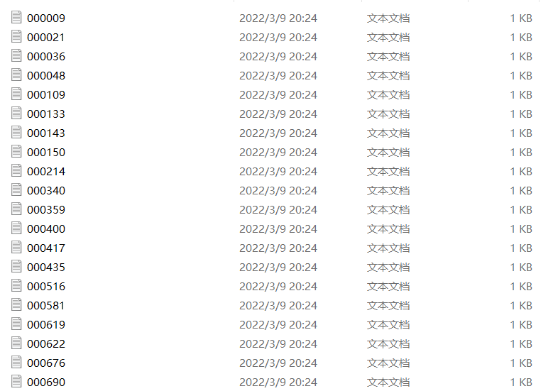
首先存放数据集的地方应该有两个部分，一个是images，一个是labels

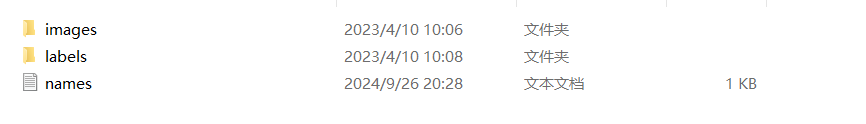
images文件夹用来存放原始的图片数据，包括训练集和测试集，而labels文件夹则是对应的标签

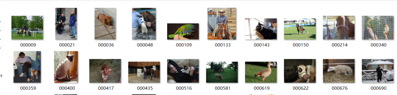
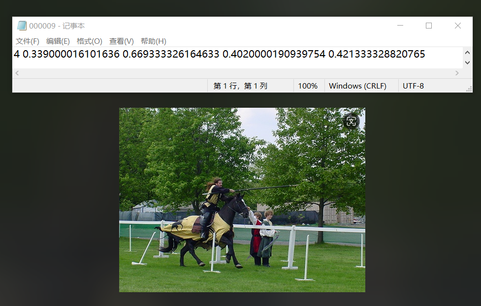
这个标签文件一共是由五个部分组成，因为图中只有一个动物，所以标签内只有一行，标签每一行第一个数字代表是类别，在这个示例中，动物是马所以是4，第二个和第三个数字代表是标记框的中心点的x，y的坐标，而后面两个数字代表的是标记框的长，宽，这些数字做过归一化的处理，所以是0~1之间的数字。按照这个标准来放置数据，可以为后续训练提供方便。如果你需要使用自己的数据集，那么就需要对图片进行标注。

对图片进行标注

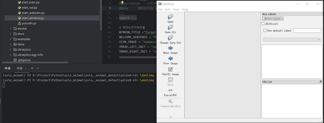
在pycharm终端中，输入labelimg，启动标注软件

注意！在这里标注的图像一定要是英文路径，最好是一次标注完，这样标签不会产生错位

点击Change Save Dir选择你存放的文件夹路径，再点击Open Dir打开存放原始图片的文件

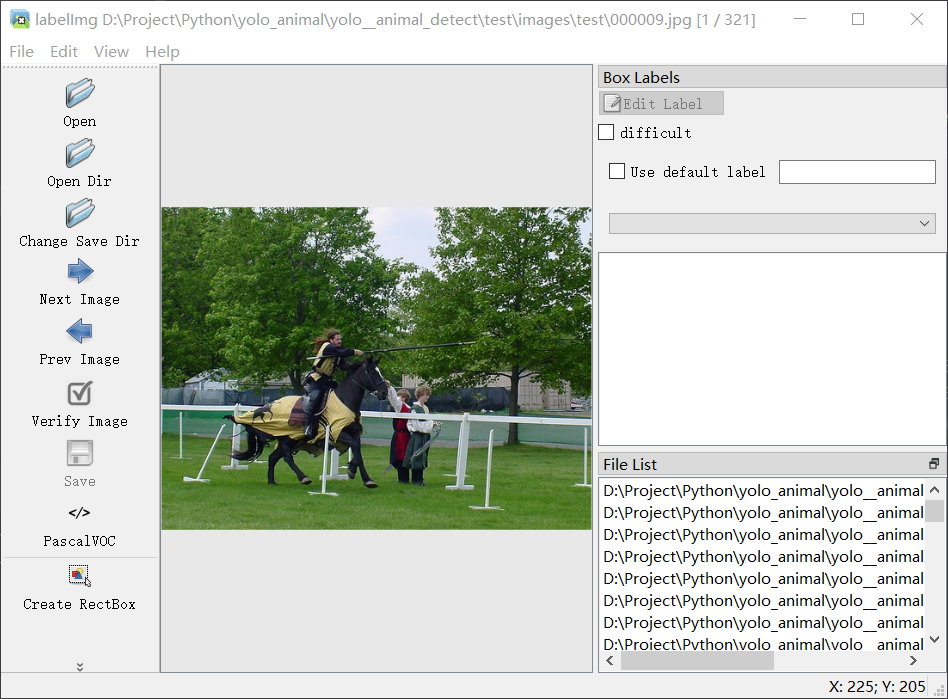
点击Pascal VOC将转换的格式改成yolo，然后点击Create RectBox开始标框，并注明类别，每完成一个酒店及Next Image切换到下一张图片，对应的存放标签的文件就会存放标签，而classes.txt文件则存放着你的标签种类，顺序一定不能变，因为这个和你的标签文件是一一对应的

模型训练和模型测试

在ultralytics目录找到配置文件，将路径修改完成（根目录、训练集、测试集等）

# Train/val/test sets as 1) dir: path/to/imgs, 2) file: path/to/imgs.txt, or 3) list: [path/to/imgs1, path/to/imgs2, ..]
path: D:/Project/Python/yolo_animal/yolo__animal_detect/animal_yolo_format #绝对路径相对路径均可
train: # train images (relative to 'path')  16551 images
  - images/train
val: # val images (relative to 'path')  4952 images
  - images/val
test: # test images (optional)
  - images/test

# Classes
names:
  0: bird
  1: cat
  2: cow
  3: dog
  4: horse
  5: sheep

配置好配置文件后，回到模型的配置文件

# Ultralytics YOLO 🚀, AGPL-3.0 license
# YOLOv8 object detection model with P3-P5 outputs. For Usage examples see https://docs.ultralytics.com/tasks/detect

# Parameters
nc: 80 # number of classes
scales: # model compound scaling constants, i.e. 'model=yolov8n.yaml' will call yolov8.yaml with scale 'n'
  # [depth, width, max_channels]
  n: [0.33, 0.25, 1024] # YOLOv8n summary: 225 layers,  3157200 parameters,  3157184 gradients,   8.9 GFLOPs
  s: [0.33, 0.50, 1024] # YOLOv8s summary: 225 layers, 11166560 parameters, 11166544 gradients,  28.8 GFLOPs
  m: [0.67, 0.75, 768] # YOLOv8m summary: 295 layers, 25902640 parameters, 25902624 gradients,  79.3 GFLOPs
  l: [1.00, 1.00, 512] # YOLOv8l summary: 365 layers, 43691520 parameters, 43691504 gradients, 165.7 GFLOPs
  x: [1.00, 1.25, 512] # YOLOv8x summary: 365 layers, 68229648 parameters, 68229632 gradients, 258.5 GFLOPs

# YOLOv8.0n backbone
backbone:
  # [from, repeats, module, args]
  - [-1, 1, Conv, [64, 3, 2]] # 0-P1/2
  - [-1, 1, Conv, [128, 3, 2]] # 1-P2/4
  - [-1, 3, C2f, [128, True]]
  - [-1, 1, Conv, [256, 3, 2]] # 3-P3/8
  - [-1, 6, C2f, [256, True]]
  - [-1, 1, Conv, [512, 3, 2]] # 5-P4/16
  - [-1, 6, C2f, [512, True]]
  - [-1, 1, Conv, [1024, 3, 2]] # 7-P5/32
  - [-1, 3, C2f, [1024, True]]
  - [-1, 1, SPPF, [1024, 5]] # 9

# YOLOv8.0n head
head:
  - [-1, 1, nn.Upsample, [None, 2, "nearest"]]
  - [[-1, 6], 1, Concat, [1]] # cat backbone P4
  - [-1, 3, C2f, [512]] # 12

  - [-1, 1, nn.Upsample, [None, 2, "nearest"]]
  - [[-1, 4], 1, Concat, [1]] # cat backbone P3
  - [-1, 3, C2f, [256]] # 15 (P3/8-small)

  - [-1, 1, Conv, [256, 3, 2]]
  - [[-1, 12], 1, Concat, [1]] # cat head P4
  - [-1, 3, C2f, [512]] # 18 (P4/16-medium)

  - [-1, 1, Conv, [512, 3, 2]]
  - [[-1, 9], 1, Concat, [1]] # cat head P5
  - [-1, 3, C2f, [1024]] # 21 (P5/32-large)

  - [[15, 18, 21], 1, Detect, [nc]] # Detect(P3, P4, P5)

最上面的nc是类别数目，会根据数据集改变，不需要专门更改

有了配置文件后可以开始进行训练了

import time
from ultralytics import YOLO


# yolov8n模型训练：训练模型的数据为'A_my_data.yaml'，轮数为100，图片大小为640，设备为本地的GPU显卡，关闭多线程的加载，图像加载的批次大小为4，开启图片缓存
model = YOLO('yolov8n.pt')  # load a pretrained model (recommended for training)
results = model.train(data='A_my_data.yaml', epochs=100, imgsz=640, device=[0,], workers=0, batch=4, cache=True)  # 开始训练
time.sleep(10) # 睡眠10s，主要是用于服务器多次训练的过程中使用
# yolov3n模型训练：
model = YOLO('../../pretrained/yolov8s.pt')  # load a pretrained model (recommended for training)
results = model.train(data='A_my_data.yaml', epochs=100, imgsz=640, device=[0,], workers=0, batch=4, cache=True)  # 开始训练
time.sleep(10) # 睡眠10s，主要是用于服务器多次训练的过程中使用
# yolov5l模型训练：
model = YOLO('../../pretrained/yolov9s.pt')  # load a pretrained model (recommended for training)
results = model.train(data='A_my_data.yaml', epochs=100, imgsz=640, device=[0,], workers=0, batch=4, cache=True)  # 开始训练
time.sleep(10) # 睡眠10s，主要是用于服务器多次训练的过程中使用
# yolov8l模型训练：
model = YOLO('../../pretrained/yolov10s.pt')  # load a pretrained model (recommended for training)
results = model.train(data='A_my_data.yaml', epochs=100, imgsz=640, device=[0,], workers=0, batch=4, cache=True)  # 开始训练
time.sleep(10) # 睡眠10s，主要是用于服务器多次训练的过程中使用

训练结束后一般会得到一系列文件，其中weights文件夹下best.pt和last.pt分别代表最佳和最后的模型，args.yaml是参数文件，还有些关于模型评价的图片

然后验证模型

from ultralytics import YOLO

# 加载自己训练好的模型，填写相对于这个脚本的相对路径或者填写绝对路径均可
model = YOLO("runs/detect/yolov8n/weights/best.pt")

# 开始进行验证，验证的数据集为'A_my_data.yaml'，图像大小为640，批次大小为4，置信度分数为0.25，交并比的阈值为0.6，设备为0，关闭多线程（windows下使用多线程加载数据容易出现问题）
validation_results = model.val(data='A_my_data.yaml', imgsz=640, batch=4, conf=0.25, iou=0.6, device="0", workers=0)

模型预测和图形化界面开发

拿到训练完的模型后，就可以进行后续的开发了

比如做一个预测的脚本

from ultralytics import YOLO

# Load a model
model = YOLO("yolov8n.pt")  # pretrained YOLOv8n model

# Run batched inference on a list of images
results = model(["images/resources/demo.jpg", ])  # return a list of Results objects

# Process results list
for result in results:
    boxes = result.boxes  # Boxes object for bounding box outputs
    masks = result.masks  # Masks object for segmentation masks outputs
    keypoints = result.keypoints  # Keypoints object for pose outputs
    probs = result.probs  # Probs object for classification outputs
    obb = result.obb  # Oriented boxes object for OBB outputs
    result.show()  # display to screen
    result.save(filename="images/resources/result.jpg")  # save to disk

除此以外还可以基于pyside6进行图形化开发